This post was inspired by the video series, 4 Essential Microsoft Excel Skills Every Marketer Should Learn. If you want to become a master of the almighty spreadsheet, watch the full video series here.
I know, "VLOOKUP function" sounds like the geekiest, most complicated thing ever. But by the time you finish reading this article, you'll wonder how you ever survived in Excel without it.
As was the case with pivot tables, Microsoft Excel's VLOOKUP function is easier to use than you think. What's more, it is incredibly powerful, and is definitely something you want to have in your arsenal of analytical weapons. What does VLOOKUP do, exactly? Here's the simple explanation: The VLOOKUP function searches for a specific value in your data, and once it identifies that value, it can find -- and display -- some other piece of information that's associated with that value.
VLOOKUP Example
You could use the VLOOKUP formula to transfer revenue data from a separate spreadsheet and match it with the appropriate customer based on a common identifier like a customer ID or email address. In this example, VLOOKUP enables you to easily see revenue by customer without searching, copying, and pasting for each individual cell.
In practical terms, this means you can take the revenue data from your second spreadsheet and integrate it with the customer data in your first spreadsheet in order to reveal the bigger picture about your business's performance.
Below, you'll see a five-step guide to performing this VLOOKUP example, followed by a video tutorial for using VLOOKUP to organize a list of blog posts.
How does VLOOKUP work?
VLOOKUP stands for "vertical lookup." In Excel, this means the act of looking up data vertically across a spreadsheet, using the spreadsheet's columns -- and a unique identifier within those columns -- as the basis of your search. When you look up your data, it must be listed vertically wherever that data is located.
The formula always searches to the right.
When conducting a VLOOKUP in Excel, you're essentially looking for new data in a different spreadsheet that is associated with old data in your current one. When VLOOKUP runs this search, it always looks for the new data to the right of your current data.
For instance, if one spreadsheet has a vertical list of names, and another spreadsheet has an unorganized list of those names and their email addresses, you can use VLOOKUP to retrieve those email addresses in the order you have them in your first spreadsheet. Those emails addresses must be listed in the column to the right of the names in the second spreadsheet, or Excel won't be able to find them. (Go figure ... )
The formula needs a unique identifier to retrieve data.
The secret to how VLOOKUP works? Unique identifiers.
A unique identifier is a piece of information that both of your data sources share, and -- as its name implies -- it is unique (i.e. the identifier is only associated with one record in your database). Unique identifiers include product codes, stock keeping units (SKUs), and customer contacts.
Since CRMs like HubSpot use email addresses to uniquely identify the contacts in their databases, HubSpot customers can use "email address" as their unique identifier to execute a VLOOKUP.
How to Use VLOOKUP in Excel
- Identify a column of cells you'd like to fill with new data.
- Select 'Function' (Fx) > VLOOKUP and insert this formula into your highlighted cell.
- Enter the lookup value for which you want to retrieve new data.
- Enter the table array of the spreadsheet where your desired data is located.
- Enter the column number of the data you want Excel to return.
- Enter your range lookup to find an exact or approximate match of your lookup value.
- Click 'Done' (or 'Enter') and fill your new column.
Take the VLOOKUP example above. Let's say you're looking through your HubSpot data and are checking out which of your site pages your contacts have viewed. You're also paying attention to whether or not any of those contacts have converted into customers.
Then it hits you: In addition to knowing which of those contacts have closed, you want to know how much MRR (monthly recurring revenue) each of them brings in. That way, you can tie your revenue back to your site pages and do some analysis to see which pages are having the biggest impact on your bottom line.
There's only one problem: Your MRR data lives in your CRM. And while you could manually look up each and every contact in your CRM to find their MRR, and then manually match those values to their corresponding contacts in your HubSpot data, the whole process would be ridiculously time-consuming and impractical.
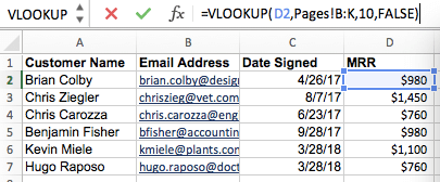
That's where the VLOOKUP function comes in. For your reference, here's what a VLOOKUP function looks like:
VLOOKUP(lookup_value , table_array , col_index_num , range_lookup)
In the steps below, we'll assign the right value to each of these components, using customer names as our unique identifier to find the MRR of each customer.
1. Identify a column of cells you'd like to fill with new data.
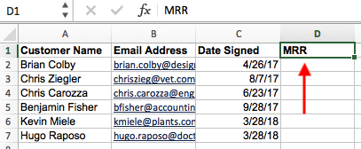
If this data is coming from a pivot table made in Excel, copy the data into a new spreadsheet so the VLOOKUP function can freely read this data.
Then, label a column next to the cells you want more information on with a proper title in the top cell, such as "MRR," for monthly recurring revenue. This new column is where the data you're fetching will go.
2. Select 'Function' (Fx) > VLOOKUP and insert this formula into your highlighted cell.
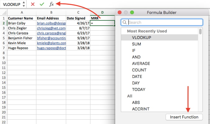
To the left of the text bar above your spreadsheet, you'll see a small function icon that looks like a script "Fx." Click on the first empty cell beneath your column title and then click this function icon. A box titled "Formula Builder" will appear to the right of your screen.
Select "VLOOKUP" from the list of options included in the Formula Builder. Then, select "Insert Function" at the bottom of this list. The cell you currently have highlighted in your spreadsheet should now look like this: "=VLOOKUP()"
You can also enter this formula into a call manually by entering the bold text above exactly into your desired cell.
3. Enter the lookup value for which you want to retrieve new data.
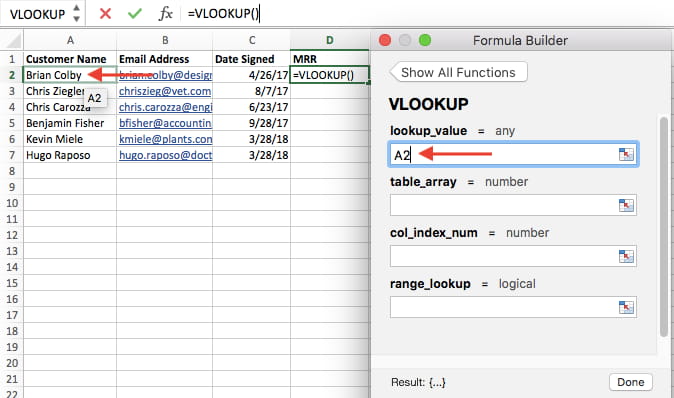
With the =VLOOKUP text entered into your first cell, it's time to fill the formula with four different criteria. These criteria will help Excel narrow down exactly where the data you want is located and what to look for.
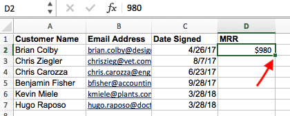
The first criteria is your lookup value -- this is the value of your spreadsheet that has data associated with it, which you want Excel to find and return for you. To enter it, click on the cell that carries a value you're trying to find a match for. In our example, shown above, it's in cell A2. You'll start migrating your new data into D2, since this cell represents the MRR of the customer name listed in A2.
Keep in mind your lookup value can be anything: text, numbers, website links, you name it. As long as the value you're looking up matches the value in the referring spreadsheet -- which we'll talk about that in the next step -- this function will return the data you want.
4. Enter the table array of the spreadsheet where your desired data is located.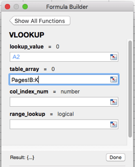
Next to the "table array" field, enter the range of cells you'd like to search and the sheet where these cells are located, using the format shown in the screenshot above. The entry above means the data we're looking for is in a spreadsheet titled "Pages" and can be found anywhere between column B and column K.
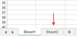
The sheet where your data is located must be within your current Excel file. This means your data can either be in a different table of cells somewhere in your current spreadsheet, or in a different spreadsheet linked at the bottom of your workbook, as shown below.
For example, if your data is located in "Sheet 2" between cells C7 and L18, your table array entry will be "Sheet2!C7:L18."
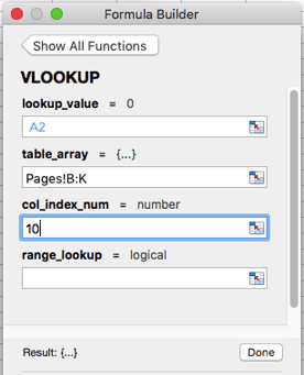
5. Enter the column number of the data you want Excel to return.
Beneath the table array field, you'll enter the "column index number" of the table array you're searching through. For example, if you're focusing on columns B through K (notated "B:K" when entered in the "table array" field), but the specific values you want are in column K, you'll enter "10" in the "column index number" field, since column K is the 10th column from the left.
6. Enter your range lookup to find an exact or approximate match of your lookup value.
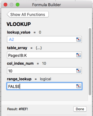
In situations like ours, which concerns monthly revenue, you want to find exact matches from the table you're searching through. To do this, enter "FALSE" in the "range lookup" field. This tells Excel you want to find only the exact revenue associated with each sales contact.
To answer your burning question: Yes, you can allow Excel to look for an approximate match instead of an exact match. To do so, simply enter TRUE instead of FALSE in the fourth field shown above.
When VLOOKUP is set for an approximate match, it's looking for data that most closely resembles your lookup value, rather than data that is identical to that value. If you're looking up data associated with a list of website links, for example, and some of your links have "https://" at the beginning, it might behoove you to find an approximate match just in case there are links that do not have this "https://" tag. This way, the rest of the link can match without this initial text tag causing your VLOOKUP formula to return an error if Excel can't find it.
7. Click 'Done' (or 'Enter') and fill your new column.
In order to officially bring in the values you want into your new column from Step 1, click "Done" (or "Enter," depending on your version of Excel) after filling the "range lookup" field. This will populate your first cell. You might take this opportunity to look in the other spreadsheet to make sure this was the correct value.
If so, populate the rest of the new column with each subsequent value by clicking the first filled cell, then clicking the tiny square that appears on the bottom-right corner of this cell. Done! All your values should appear.
Alright, enough explanation: let's see another example of the VLOOKUP in action!
In the video below, we're taking the pivot table we made in video #2, pasting the values into a new sheet, and using it as an example report. We then use the VLOOKUP function to match blog post authors (from our second data source) to their corresponding post titles. In this instance, we're using post title as our unique identifier.
Author's note: There are many different versions of Excel, so what you see in the video above might not always match up exactly with what you'll see in your version. That's why we encourage you to download the written instructions and demo data so you can follow along.
Download demo data | Download instructions (Mac) | Download instructions (PC)
Want to learn to do more in Excel? Download the full video series, 4 Essential Microsoft Excel Skills Every Marketer Should Learn.


No comments:
Post a Comment